In this article, we will discuss the history, current usage, and development of Neural Networks. We will try to understand each of the segments while visualizing them.

This article aims to introduce neural networks in a manner that will require little to no prerequisites from the reader about the topics.

Chapter 1: Introduction to Neural Networks

Part 1: PERCEPTRONS

1.0 VISUALISING PERCEPTRON

It all started in 1958 with the invention of Perceptron. It was an algorithm that was used to mimic the biological neuron. A perceptron was a type of Artificial Neuron.

You might have seen the following figure in your school biology textbooks. So, what does it have to do with perceptron?!

Let’s see how a perceptron relates to a biological neuron.

If you observe the above image you will notice quite some similarities between a biological neuron and an artificial neuron.

Both take some input from the left-hand side and then process the data(applying the logic) in the middle part of it and then produces an output.

Take a look at the above animation for 2-3 iterations and you will be able to understand it well enough.

Although, in reality, artificial neurons are nothing like biological neurons, they are just inspired you can say.

1.1 WORKING OF THE PERCEPTRON

Now we know how a perceptron looks, let’s see how it works.

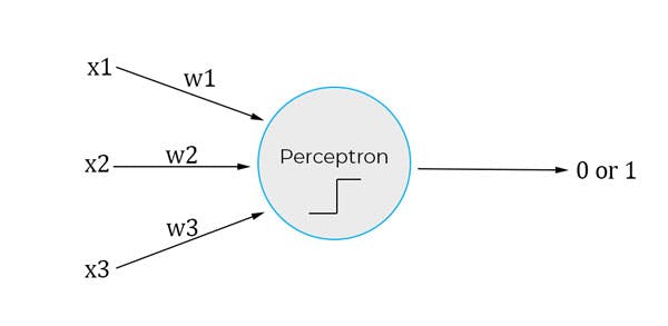
Perceptron accepts only binary input i.e., 1 or 0 and similarly, it also outputs in binary. So, if x1, x2, and x3 are input to a perceptron they all can be either a 1 or 0.

Do you see those w1, w2, and w3 in the image? Those are called “weights”, we will talk about them in a bit.

The perceptron works by taking the sum of inputs with the product of their respective weights and then comparing it to the threshold value, so the output is 0, 1 depending on whether the weighted sum( ∑wi.xi ) is greater or less than the threshold value. So, the output of the above figure will be determined by ∑wi.xi = “x1.w1 + x2.w2 + x3.w3” which is then compared to the threshold value to produce output.

Mathematically, it is easier to understand:

$$\sum_{i}w_i.x_i=x1w1+x2w2+x3w3$$

$$\text{output}= \begin{cases} \text{0 if }\sum\limits_i w_i.x_i \le\text{threshold} \cr\text{1 if }\sum\limits_i w_i.x_i >\text{threshold} \end{cases}$$

Now to understand perceptron we shall take an example, this example may not be a real application but it will help us understand perceptron easily.

Now, suppose you want to go to watch a football match this weekend in a stadium in your city. But the tickets are expensive. There are three conditions that determine whether you will go to watch the match or not:

x1: Do you have enough money to buy the ticket?

x2: Is your favourite team playing?

x3: Is the weather good?

If you were to feed these conditions into the perceptron they can only be 0 or 1.

So, let’s say you have enough money to buy the ticket you will set “x1 = 1” otherwise you will set “x1 = 0” and if your favourite team is playing set “x2 = 1” otherwise set “x2 = 0” and if the weather is good enough to go out set “x3 = 1” else set “x3 = 0”.

Before, feeding these conditions in the perceptron we will also have to adjust “weights”.

So, what are “weights”? In simple words, weights are the importance you give to your input conditions.

So, let’s say the most important condition for you to go watch the match is whether you have money to buy the ticket, because if you don’t have the money you cannot buy the ticket, so you will assign a greater value of weight to it, let’s say w1 = 5.

Now, you also care about whether your favourite team is playing or not, so you assign a weight of w2 = 2 to it.

But, you don’t care if the weather is good or bad, you are a big football fan and you will still go, so you assign a relatively small weight to that, let’s say w3 = 1.

Now, when you put this in equation 1 and equation 2, you will see if you don’t have the money the output will always be 0 even if your favourite team is playing and the weather is good (assuming the threshold to be 3.5). This is because you have assigned the largest weight to w1. And, if you have the money to buy the tickets the perceptron will most probably output 1.

This is how weights are used in perceptron to set the importance or weightage of any input. Also, just like weights, the threshold value is adjusted manually according to the need.

As you have observed, the reason why the perceptron outputs only 0 or 1 is the threshold value which arises due to the usage of the step function.

The step function is used in perceptron, you can see the step function diagrammatically below, and you should be able to understand how it works with perceptron.

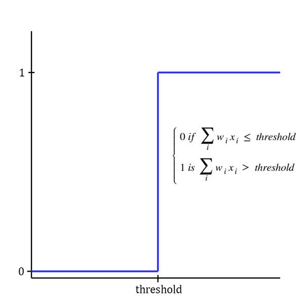
As we can observe, due to step function as-soon-as the output is greater than the threshold value perceptron outputs 1 and for any value equal or less than the threshold, perceptron outputs 0.

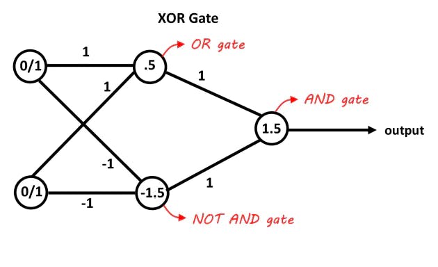
By using perceptrons we could build a network to solve any logic, which in turn made perceptrons another form of logic gates. Why would we need another form of logic gates when we already had those? This issue stalled the development and the funding of perceptrons.

Using the step function resulted in the biggest drawback of the perceptrons. This issue never allowed perceptrons to learn by changing the weights during the execution.

Later on, we realised that other types of functions can be used in neurons, and that lead to the development of the Sigmoid Neuron.

Part 2: MODERN NEURONS

2.0 DIFFERENCE BETWEEN MODERN NEURONS AND PERCEPTRONS

Modern neurons are nothing but a slightly improved version of perceptrons, there are two major differences between any modern neuron and a perceptron:

• The output is any fractional value between 0 and 1 unlike perceptrons, which only have two outputs 0 or 1.

• We use various other Activation Functions* instead of using step function as in perceptron.

• A new term bias\** is added to the weighted sum and the threshold value is replaced by a 0.

*******The functions used in neurons to implement the logic are called Activation Functions so the step function is the activation function of the perceptron and the sigmoid function is the activation function of the sigmoid neuron.

********The threshold value in the equation(∑wi.xi ≥ threshold) is moved to the left of the equation and named “bias” (∑wi.xi + b ≥ 0).
(b ≅ – threshold).

$$output = \begin{cases}0:if:\sum\limits{i} w{i}.x{i} + b \ge 0 \1:if:\sum\limits{i} w{i}.x{i} + b < 0\end{cases}$$

Also, we are setting a new variable “z” to our weighted sum of inputs + bias to make it better to use in formulas:

$$z = \sumi w{i}.x_{i}+b$$

2.1 SIGMOID NEURONS

We have discussed above how a modern neuron is different from a perceptron, now we will talk about how this modern neuron is working better using sigmoid or other activation functions.

We now know all the theory of how a sigmoid neuron is better than a perceptron but I think it’s all a waste until we visualise it, so let’s dive into how a sigmoid function works to understand how it makes a sigmoid neuron more viable than a perceptron.

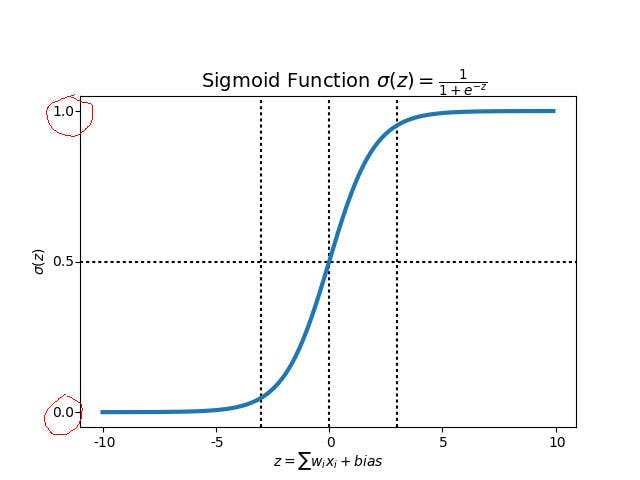
The above figure shows you how a sigmoid function looks. Unlike, the step function sigmoid function has a much smoother slope.

If you observe Fig 2 above, on the left(marked with red), the sigmoid function(in blue) goes from 0 to 1. Hence, for any input, it gives an output between 0 and 1.

Now, let’s try and understand this mathematically. The formula for the sigmoid function is given as:

$$sigmoid(z) = \sigma(z) = \frac{1}{1+e^{-z}}$$

We will discuss two cases to understand the sigmoid function.

• When the value of “z” is a very large number.

$$\sigma(large:number) = \frac{1}{1+e^{-(large:number)}} =\frac{1}{1+0} = 1$$

• When the value of “z” is a very large NEGATIVE number.

$$\sigma(large:negative:number) = \frac{1}{1+e^{-(large:negative:number)}} =\frac{1}{1+\infty} = 0$$

The above two equations show that for very large or very small values the output of the sigmoid function is 1 and 0 respectively and for other values, the sigmoid function gives values between 1 and 0.

So, a sigmoid neuron will look something like this diagrammatically:

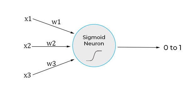
It looks very similar to the perceptron we have seen above, just changing the activation function and outputs.

Part 3: NEURAL NETWORKS

3.0 WHAT IS AN ARTIFICIAL NEURAL NETWORK(ANN)

After understanding Neurons we can take a look at what a Neural Network(NN) is, in simple words, we can say that:

“An Artificial Neural Network is a network of artificial neurons”

When we interconnect two or more neurons with each other, that can be called a neural network.

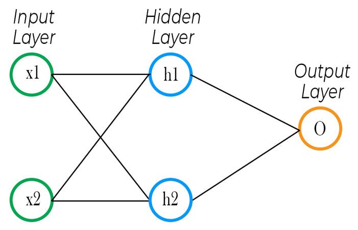
In the above figure, we can see a simple ANN, it consists of 2 layers(because we don’t count the input layer). The input layer gives input to the hidden layer, it’s called a hidden layer because it is neither input or an output layer, the output of the hidden layer is fed into the output layer which computes our final calculation.

If this is a bit tricky to understand don’t worry, we will discuss how an ANN works in detail in the next chapter.

An ANN is also called simply a Neural Network.

3.1 ARCHITECTURE OF A NEURAL NETWORK

The Neural Networks are designed to resemble the human brain, the ANNs are a simple model that is formed by joining the appropriate number of neurons in order to solve a classification problem or to find patterns in the data.

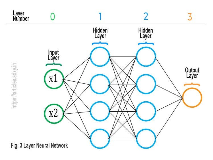
In the above figure, we can observe a 3-layer Neural Network. As we can observe there is one input layer, two hidden layers, and one output layer.

This is a three-layered Neural Network because we never count the Input Layer to be a part of the Neural Network layers.

The hidden layers are called hidden just because they are neither the input layer nor the output layer. Or, we can say that the user doesn’t interact with the hidden layer directly and therefore it is called a hidden layer.

Any number of layers having any number of neurons can be used in any respective layer to achieve the desired goal. For example, the output layer can have two or more neurons instead of one for any different neural network.

This concludes the Introduction to Neural Networks, to read more about these topics follow some of the references below.

References:

• Comprehensive Introduction to Neural Network Architecture

• Neural Networks and Deep Learning online book by Michael Nielsen